5. Left-Ventricle Segmentation

This chapter covers PredictSegmentation.py — the all-in-one script that segments the left ventricle in echocardiogram videos and .npy frames.

5.1. Configure the paths

Edit the configuration block near the top of PredictSegmentation.py:

INPUT_DIR  = r"...\EchoNet-dynamic\demo\video"
WEIGHTS    = r"...\EchoNet-dynamic\stats\deeplabv3_resnet50_random.pt"
OUTPUT_DIR = r"...\EchoNet-dynamic\demo_output"

Variable	Meaning
`INPUT_DIR`	Folder scanned for `.avi`/`.mp4` videos and `.npy` frames
`WEIGHTS`	DeepLabV3-ResNet50 checkpoint (`stats\deeplabv3_resnet50_random.pt`)
`OUTPUT_DIR`	Folder where all results are written (created automatically)

To run on your own clips, point INPUT_DIR at your folder. OUTPUT_DIR is created automatically.

The script also reads the MEAN/STD block at the top of the file. Both the image (.npy) and video modules now use the same statistics. Keep the defaults for EchoNet-style data, or recompute them for your own dataset — see Normalization Statistics.

5.2. Run the script

conda activate echonet
python scripts/PredictSegmentation.py

The script prints the device it is using:

🚀 Running device: cuda
🧠 Loading DeepLabV3 model onto GPU...
📁 Scan complete: found 1 videos and 0 .npy files.

GPU vs CPU

If no GPU is found it falls back to CPU automatically and warns you. CPU works but is much slower because the video module does frame-by-frame inference.

5.3. What happens under the hood

5.3.1. Model

model = torchvision.models.segmentation.deeplabv3_resnet50(pretrained=False, aux_loss=False)
model.classifier[-1] = torch.nn.Conv2d(..., 1, ...)   # 1 output channel = LV mask

The checkpoint’s state_dict is loaded, stripping any module. prefix left over from multi-GPU training.

5.3.2. Module A — `.npy` frames

For each .npy file the script:

Normalises the array to a 112 × 112 RGB image.
Applies the configured MEAN/STD normalisation and runs the model.
Builds a mask where the model output is positive (pred > 0).
Computes LV area as the number of mask pixels.
Saves a 448×448 layout image — the original and the green-masked image side by side, with the LV area printed underneath — into segmentation_images/, named <name>_segmentation.png.
Appends a row to image_lv_area.csv.

5.3.3. Module B — videos

For each video the script:

Reads and resizes every frame to 112 × 112.
Runs the model in batches of 20 frames to limit memory use.
Computes the LV area (size) for every frame.
Detects systole frames as the troughs (negative peaks) of the area curve using scipy.signal.find_peaks — peaks at least 20 frames apart, with a prominence of 50 % of the spread between the n**0.05 and n**0.95 order statistics of the per-frame sizes (the original EchoNet heuristic, not the 5th/95th percentiles).
Writes an annotated <name>_segmentation.avi (original + red LV overlay
- a moving white size trace) into segmentation_videos/ using echonet.utils.savevideo.
Saves a <name>_area_curve.pdf plot of LV size vs. time with systole markers into area_curves/.
Appends one row per frame to video_lv_area.csv.

Systole detection needs enough frames

Peak detection only runs when a video has more than 10 frames. Very short clips will simply report sizes with no systole flags.

5.4. Outputs

After a run, OUTPUT_DIR contains (sub-folders are created on demand — you only get the ones relevant to your inputs):

OUTPUT_DIR/
├── segmentation_videos/    # <name>_segmentation.avi   annotated videos
├── area_curves/            # <name>_area_curve.pdf      LV area-vs-time curves
├── segmentation_images/    # <name>_segmentation.png    per-image mask layouts
├── video_lv_area.csv       # Filename, Frame, Size, ComputerSystole
└── image_lv_area.csv       # Filename, LV_Area_Pixels(112x112_scale), Status

5.4.1. Example outputs

Here is what PredictSegmentation.py produced on the bundled demo.

Video (Module B) — the annotated clip overlays the LV in red and draws a moving white trace of the area curve; the grey band marks detected systole:

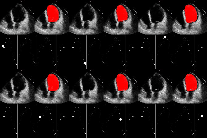
../_images/segmentation_demo.gif — Fig. 5.4.1 `segmentation_videos/0X243FDE8AE0A05B6F_segmentation.avi`, shown here as a GIF.

The matching area curve is roughly periodic, with the three detected systole frames (32, 75, 119) marked by dashed lines:

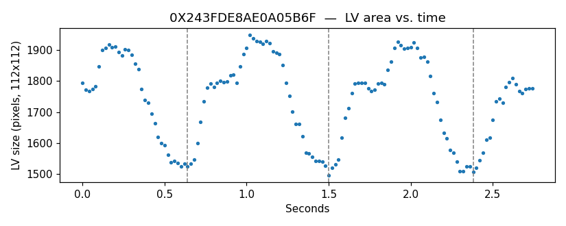
../_images/area_curve.png — Fig. 5.4.2 `area_curves/0X243FDE8AE0A05B6F_area_curve.pdf`.

Single frame (Module A) — each .npy frame becomes an original-vs-mask layout with the LV area printed underneath:

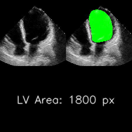
../_images/seg_frame_0046.png — Fig. 5.4.3 `segmentation_images/frame_0046_segmentation.png` (LV area 1800 px).

5.4.2. `video_lv_area.csv` columns

Column	Meaning
`Filename`	Source video name
`Frame`	Frame index (0-based)
`Size`	LV area in pixels at that frame (112×112 scale)
`ComputerSystole`	`1` if the frame was detected as systole, else `0`

5.4.3. `image_lv_area.csv` columns

Column	Meaning
`Filename`	Source `.npy` name
`LV_Area_Pixels(112x112_scale)`	LV area in pixels
`Status`	Always `Success`; unreadable or unsupported `.npy` files are skipped with a console warning and get no row

See Results & Troubleshooting for how to interpret and verify these outputs.